Having introduced the mathematical and statistical background for the main topic, we still have to introduce a fundamental model of unsupervised learning called K-Means. K-Means is an unsupervised clustering algorithm to partition unlabelled data into different clusters. More formally, suppose we have a dataset: {x1, x2, …, xN} consists of N observations of a random D-dimensional Euclidean variable x, the goal of the K-Means algorithm is to partition the data into some number K of clusters.
To be more specific, we can have the following example to partition the data into 2 classes:
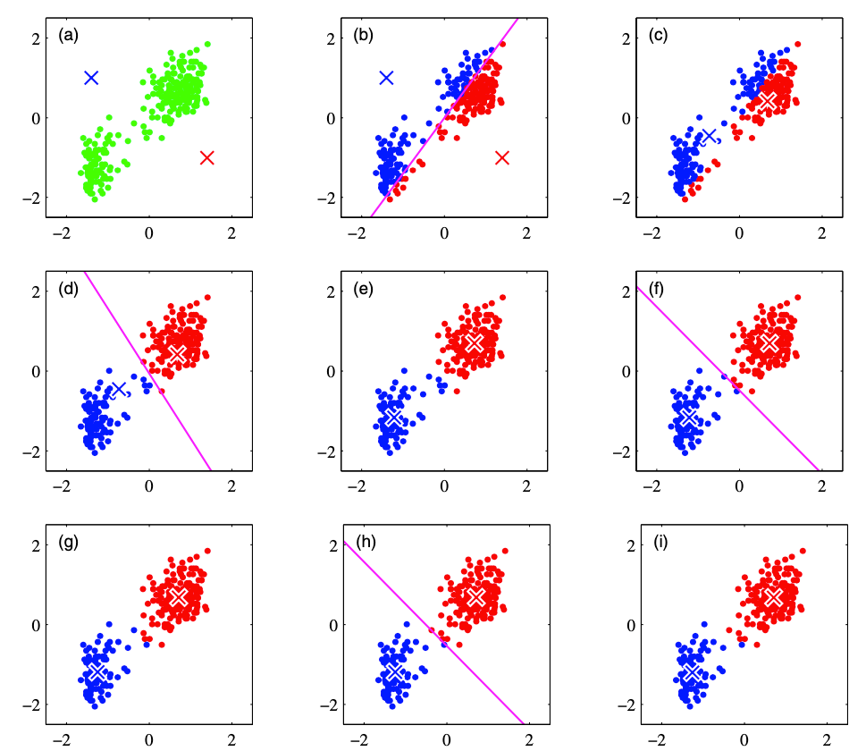
From (a) to (i), the plots demonstrate how the K-Means algorithm works. K-Means is an iterative approach that first (1) initialize K cluster centers. Then (2) it assigns each point to the specific cluster based on the squared distance to the cluster center. After that, (3) all the points in the same cluster will decide the new cluster center. The new cluster centers of each cluster are calculated by the average of all data points in that cluster. It is therefore called K-Means algorithm. The above step (2) and step (3) will be performed iteratively until there is no further update of the cluster centers.
Mathematically, the process of the K-Means algorithm can be described as follows:
Optimization process: find values for {rnk} and {𝜇k} to minimize J (for each n in 1, 2, …, N, k in 1, 2, …, K)
Objective function:
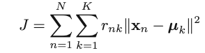
Initialization: choose K and initial {𝜇k}
Iterative steps:
Iterative step 1: Minimize J w.r.t. {rnk} , with {𝜇k} fixed: [re-assign data points]
![]()
2. Iterative step 2: Minimize J w.r.t. {𝜇k}, with {rnk} fixed: [re-compute cluster means] First of all, take the derivative of the objective function w.r.t. 𝜇k
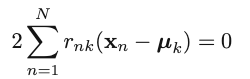
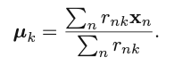
We can then obtain the optimal update for the current 𝜇k:
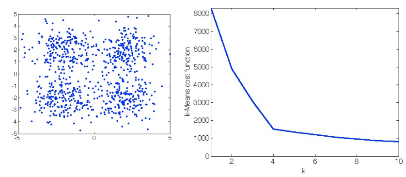
The two-phase iteration is performed until there is no change in {rnk} and {𝜇k}. This algorithm guarantees a monotonic decrease of the objective function, and it is guaranteed to find a local optimum. But the k should be determined prior to the execution of the algorithm. The following figure shows how different choices of K influences the cost function, based on the data points provided in the left subplot. Usually, we choose the K that would not lead to a sharp decrease of the objective function anymore (if we further increase it). For example, in the right subplot, we can see the decrease of the cost function becomes relatively flat when K is increased from 4 to 5. So, K=4 would be the best setting, in this case, to guarantee a satisfactory value in the cost function, as well as to achieve desirable generalization.
The K-Means algorithm is the foundation of the E-M Algorithm. The E-M Algorithm to be introduced in the latter part of this blog is a variant of the K-Means algorithm. By varying the objective function, there are also other clustering algorithms, such as the K-Median algorithm+, to achieve different purposes.
Before formally step into the discussion of the E-M Algorithm, it is important to learn about the problem settings. Therefore, we introduce the concept of “mixture model”, as well as the definition of “latent variable” in this section.
Latent Variable
As the name suggests, latent variables are variables in a distribution that you cannot directly observe. For example, Consider a probabilistic language model of news articles, where each article x focuses on a specific topic t (eg. finance, sports, politics). So, a more accurate model is p(x | t) * p(t). The topic t is unobserved directly but introduced by us. If we are to use the more accurate model, we need to somehow obtain the distribution of t. Therefore, if we take the latent variable into consideration, our model could become more robust under different settings.
A latent variable model (LVM) p is a probability distribution over two sets of variables x, z with parameter 𝜃: p(x, z; 𝜃). x is observed at learning time in a dataset D, z is never observed and only used in the inference process. The Gaussian Mixture Model is a typical example of the latent variable model.
Gaussian Mixture Model
The most important application of latent variables is the mixture model. In this section, we focus on Gaussian Mixture Models, to give us an overview of how mixture models work.
Suppose we have the following mathematical settings, and we have k different Gaussian distributions included in the mixture model
x: 2-d data points on the coordinate.
z: which Gaussian distribution the observed x belongs to (if k Gaussian models, z can be 1, 2, …, k)
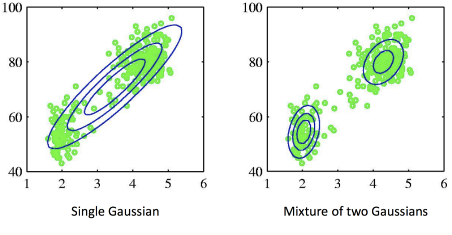
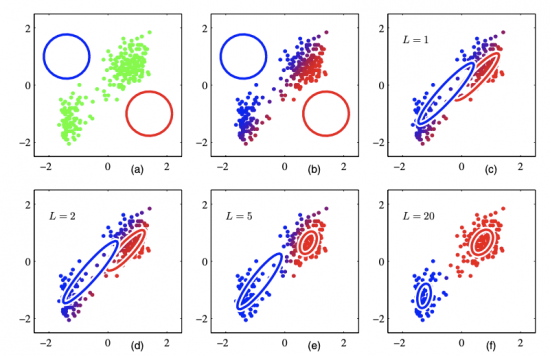
Then, the joint distribution can be represented as p(x, z) = p(x | z) p(z). We define p(z = k) = 𝜋k, and p(x | z = k) = Ɲ(x; 𝜇k, Σk), then: p(x) = ∑𝜋k Ɲ(x; 𝜇k, Σk) (where ∑𝜋k = 1, 0 <= 𝜋k <= 1, {𝜋k} is called the mixing coefficients). The following figure demonstrates the power of mixture models. If we fit the whole dataset with a mixture of two Gaussian models (see right subplot), it models the distribution of the original dataset better than one Gaussian model (see left subplot).
How can we fit a Gaussian Mixture Model into a dataset? The E-M algorithm provides a workflow.
Algorithm Step-by-Step
The full name of the E-M Algorithm is “Expectation-Maximization Algorithm”. As the name suggests, the concept of “expectation” is used during the execution of the algorithm.
To better understand the E-M Algorithm, we need to have a concrete problem setting: Consider GMM as a discrete latent variable model:
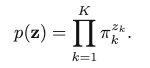
Latent variable is z (K-dimensional binary random variable, 1-of-K representation), with z = [z1, z2, …, zK]. So z only has one element equal to 1, and all other elements are 0. This is similar to the one-hot encoding scheme. Then we can define the joint distribution: p(x, z) = p(z)p(x | z). The marginal distribution is p(zk = 1) = 𝜋k. When we write z as the one-of-K encoding, the marginal distribution of z can be represented as:
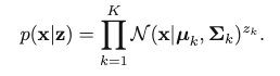
Then, we consider the conditional distribution of x given z:
which can be written with z in the vector form:
We can then have the marginal distribution of x:
So, if we want to maximize the marginal distribution, we need to maximize the log-likelihood function
![]()
where {𝜋k}, {𝜇k} and {𝛴k} are parameters of the GMM, 𝛴k = σk2 Id. If we want to maximize the log-likelihood function, we have to take the partial derivatives regarding {𝜋k}, {𝜇k} and {𝛴k}. The summation inside the log-likelihood makes the derivative intractable, non-convex and hard to reach a closed-form solution.
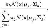
To resolve this issue, we define an important quantity, which is the posterior probability of z given observed x: 𝛾(zk) = p(zk = 1 | x), which can be calculated with Bayes’ Theorem:
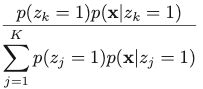
The corresponding result for Gaussian Mixture Model is:
This quantity is called “responsibility”. We encounter this quantity when we try to take the partial derivative regarding 𝜇k:
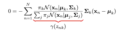
However, direct optimization of the log-likelihood is intractable. And it seems this approach does not take the advantage of “latent variable”. If the “responsibility” term is treated as a whole, the problem can become easier.
So, an alternative view of the maximization of the likelihood is that we can include the latent variable z in our model, and calculate the complete likelihood on p(x, z) instead. Maximization of the complete-data log-likelihood is more straightforward. The idea is: our knowledge of z is given by posterior p(z|x, Θ), where Θ is the set of all parameters. This term is exactly the “responsibility” term.
The complete-data likelihood can then be represented as:
And the corresponding log-likelihood is:
However, in practice, we have no idea of the value of znk because z is the latent variable whose ground-truth value can never be observed. We can only learn about z by observed x, and calculate the posterior probability:
Therefore, we can replace the value of znk by the expectation of the value of znk given x:
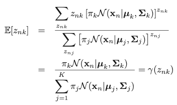
The expectation is exactly the “responsibility” term. That is how we can make use of this term in the analysis. Then, instead of maximizing the complete-data log-likelihood, we maximize its expectation, given x and the set of parameters Θ: ({𝜋k}, {𝜇k} and {𝛴k}).
So the problem becomes maximizing the above expectation of the complete-data log-likelihood. It is therefore called the “Expectation-Maximization” (EM) algorithm.
Then, we can solve the corresponding {𝜋k}, {𝜇k} and {𝛴k} by just setting the partial derivatives to 0 and solve the equations:
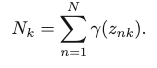
By defining Nk as the effective number of samples in the kth cluster:
We can represent the results of the current optimal update of the parameters as:
and 𝜋k = Nk / N. After having the updated parameters, we calculate the new “responsibility” for us to perform the next update of the parameters. The E-M Algorithm iteratively runs until there is no further change in the parameters. It is guaranteed to find at least a local optimum. Each update will lead to an increase of the complete-data likelihood before convergence.
A formal pseudo-code of the E-M Algorithm is as follows:
Initialization: initialize the number of mixture models K, and a parameter set for the K models
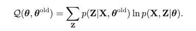
E-Step: First, Use the current parameter Θold to find the posterior distribution of latent variables p(Z | X, Θold). Then find the expectation of the complete-data log-likelihood, evaluated on some general parameter Θ:
M-Step: Θnew = argmax_Θ Q(Θ, Θold)
Steps 2 and 3 are repeated iteratively until convergence.
Below is an illustration of EM Algorithm run on the same dataset as we have previously shown in the demo of K-Means. The dataset can be partitioned in a mixture of 2 Gaussian models. The colors are continuous, indicating the posterior probability of each data point belonging to a certain cluster.
We can see there are some similarities between K-Means and EM Algorithm. Both adopt an iterative approach to find the best parameters. However, K-Means is based on geometric features (Euclidean distance), while EM Algorithm is based on statistical analysis.
Sensitivity to Initialization
EM Algorithm is sensitive to the initialization of the number of clusters and parameters. Different initialization will lead to completely different results in the final complete-data log-likelihood:
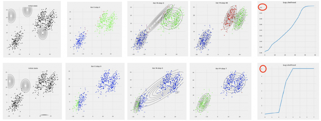
Therefore, the initialization is important. We usually run K-Means prior to running the EM Algorithm of a Gaussian Mixture Model to determine the number of clusters. The cluster centers of the GMM can be set as the cluster centers of the K-Means algorithm. The variance of the GMM is also set as the sample variance of each cluster obtained by K-Means.
Maximizing the likelihood using gradient-based methods?
Having learned about EM Algorithm, we might be curious about why we sometimes favour EM Algorithm over gradient-based methods. Gradient-based methods can also be used to maximize the likelihood function of a Gaussian Mixture Model.
In practice, EM Algorithm can be sometimes slow to reach convergence. There are situations where gradient-based methods are favoured over EM Algorithm in parameter estimations. We can have the example of the Gaussian Mixture Model again for our analysis.
As we have introduced, the maximization of the likelihood of a Gaussian Mixture Model is not a convex problem. Theoretically, using a gradient-based method can easily make the parameters get stuck in a local minimum. However, research has shown that if we want to fit a Gaussian Mixture Model on large amounts of high dimensional data, stochastic gradient descent (SGD) is superior to the traditional EM Algorithm. When the dataset gets very large, the EM Algorithm cannot be directly performed on the whole dataset. Many researchers have explored the possibility of performing the EM Algorithm for online data / in a minibatch. However, as there is no learning rate in EM Algorithm, it becomes difficult for the optimization process to be scalable to batch size. But for SGD or mini-batch gradient descent, the likelihood function can be optimized without looking at the whole dataset.
A recent study has proposed an SGD-based algorithm to tackle the abovementioned problem on a large and high-dimensional dataset. The related paper has proposed a workflow of maximizing the log-likelihood. First, we can use SGD to optimize a lower bound of the log-likelihood instead of the log-likelihood itself. Then, some enforcing mechanisms will be performed to ensure the sum of all {𝜋k} is 1. Finally, annealing procedures are introduced to avoid undesirable initial states and local minimum. This fine-tuned SGD-based algorithm on GMM outperforms EM Algorithm in some high-dimensional dataset, such as MNIST. Some results are shown in the below table:
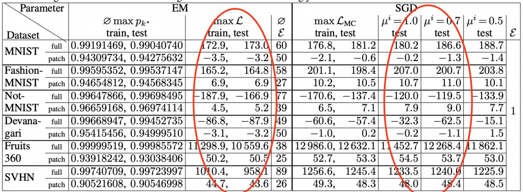
The log-likelihood values are included in the red circles. This SGD-based method outperforms EM Algorithm in almost every dataset included in the experiments. Details of this algorithm are included in reference material 3.
In the end
EM Algorithm and mixture models are the fundamentals of unsupervised learning. There have been different variants of EM Algorithm on different problems. The concept of Expectation-Maximization can be used in image segmentation, data augmentation, density estimation, and semi-supervised learning (with some data lack of labels). Therefore, it is meaningful for us to study not only supervised learning methods, but also unsupervised learning methods. Methods like K-Means and EM Algorithm are worth studying as well.
References:
Bishop, Christopher M. Pattern Recognition and Machine Learning Ch.9. Springer, 2006.
Expectation-Maximization: https://home.ttic.edu/~dmcallester/ttic101-07/lectures/em/em.pdf
Gepperth, A. and Pfülb, B. Gradient-based Training of Gaussian Mixture Models in High-Dimensional Spaces. Retrieved from: https://arxiv.org/pdf/1912.09379.pdf
Krause, Andreas. Introduction to Machine Learning, ETH Zurich: https://las.inf.ethz.ch/courses/introml-s20/tutorials/tutorial_em.pdf
Learning in Latent Variable Models:Learning in latent variable models