Method of Moments (MM) is one of the commonly-used methods to estimate parameters. It expresses the population moments as functions of the parameters of interest. And then use sample moments to estimate the population moments. Use normal distribution as an example ![]() , suppose , and we use the first two moments,
, suppose , and we use the first two moments,
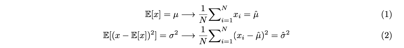
Using equation (1) and (2), we can estimate parameters ![]() and
and ![]() with
with ![]() , which are i.i.d. realizations of the random variable . By solving equations, we’re able to reach an estimation to the parameters. However, if we consider the third and fourth moments of
, which are i.i.d. realizations of the random variable . By solving equations, we’re able to reach an estimation to the parameters. However, if we consider the third and fourth moments of ![]() as well, similarly, there are two more equations.
as well, similarly, there are two more equations.
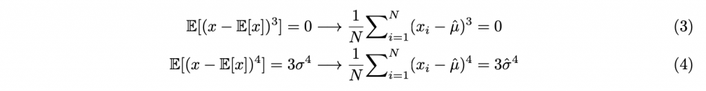
Here arise the problem, there are four equations and only two unknowns. It is referred to as over-identification problem and normally there is no solution to the system. This is where generalized method of moments works – estimating the parameters in the over-identification problem.
As Professor John Cochrane mentioned in his asset pricing course, “most of the econometrics in GMM boils down to this (standard error of the sample mean)”. We first introduce the useful results as the lemma to derive GMM.
Given a random variable ![]() , denote its sample mean as
, denote its sample mean as ![]() , we have,
, we have,
![]()
Suppose ![]() is stationary and uncorrelated, we have,
is stationary and uncorrelated, we have,
![]()
Equation (6) is the most widely seen formula for the standard error of the sample, but it requires rather strict assumptions. Now we relax the constraints, suppose ![]() is stationary but correlated, we have,
is stationary but correlated, we have,
![]()
Since ![]() is stationary, when
is stationary, when ![]() , we have an asymptotic representation of
, we have an asymptotic representation of ![]() .
.
![]()
Specifically when the mean of is 0, we have
![]()
Denote ![]() as data,
as data, ![]() as parameters that we want to estimate. Find a series of functions
as parameters that we want to estimate. Find a series of functions ![]() on
on![]() and
and ![]() .
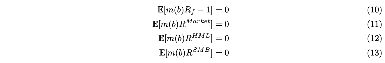
. ![]() are the population moment conditions in GMM. For example, if we consider asset pricing model using stochastic discount factors
are the population moment conditions in GMM. For example, if we consider asset pricing model using stochastic discount factors ![]() , where
, where ![]() depends on some parameter
depends on some parameter ![]() . Fama-French three factor model can be expressed as moment conditions,
. Fama-French three factor model can be expressed as moment conditions,
Denote ![]() ,where
,where ![]() meanssamplemoments. Nowsupposewe have
meanssamplemoments. Nowsupposewe have ![]() moments and
moments and ![]() parameters, when
parameters, when ![]() >
> ![]() , the question is over-identified. The central idea of GMM is to find such
, the question is over-identified. The central idea of GMM is to find such ![]() so that given a linear combinations of the sample moments, we set all such combinations equal zero. The matrix to represent the linear combination is denoted as
so that given a linear combinations of the sample moments, we set all such combinations equal zero. The matrix to represent the linear combination is denoted as ![]() , which is named “selection matrix” in Prof. Cochrane’s context. Express GMM estimator as follows,
, which is named “selection matrix” in Prof. Cochrane’s context. Express GMM estimator as follows,
![]()
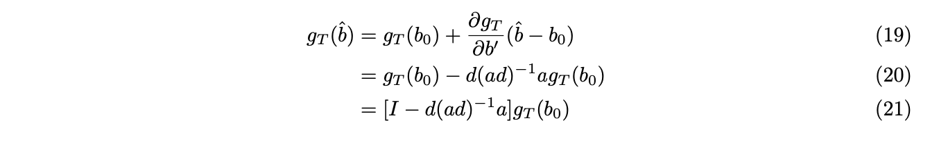
Use delta method, we apply Taylor Expansion to equation (14) at ![]()
![]()
Denote ![]() as
as ![]() ,
, ![]() is
is ![]()
![]() ×
× ![]() partial derivative matrix in numerator format. Further transform equation (15), we have,
partial derivative matrix in numerator format. Further transform equation (15), we have,
![]()
Let’s first calculate![]() . Notice that
. Notice that ![]() =
= ![]() ,
, ![]() is in fact a variance of the sample mean. Denote
is in fact a variance of the sample mean. Denote![]() , we have
, we have ![]() . Use Lemma in section 2.1, when
. Use Lemma in section 2.1, when ![]() , we have,
, we have,
![]()
Now with equation (16), we have,
![]()
Similarly, use Taylor expansion at ![]() , together with equation (16), we have,
, together with equation (16), we have,
Use the fact that![]() , we have,
, we have,
![]()
If the model is true![]() , and
, and ![]() is stationary, then
is stationary, then ![]() is consistent and asymptotic normal. We have,
is consistent and asymptotic normal. We have,
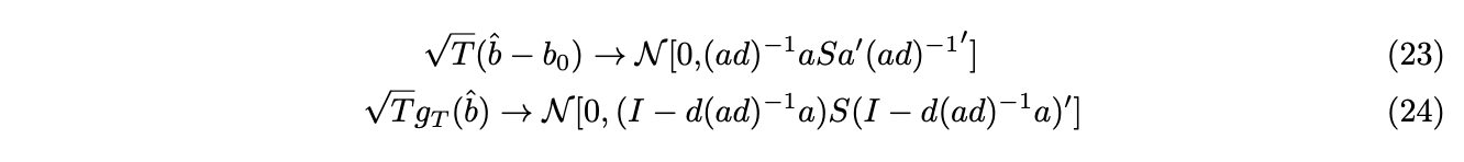
![]() evaluates the efficiency of the estimate, while
evaluates the efficiency of the estimate, while ![]() tells us how well the model is, whether the near zero result of the sample moments based on luck. Sargan-Hansen J-test can be used to test the model.
tells us how well the model is, whether the near zero result of the sample moments based on luck. Sargan-Hansen J-test can be used to test the model.
Sargan(1958) proposed tests for over-identifying restrictions based on instrumental estimators that are distributed in large samples as Chi-square variables with degree of freedom ![]() −
− ![]() . Hansen(1982) used this test in GMM estimators. Under
. Hansen(1982) used this test in GMM estimators. Under ![]() , the model is valid, while under
, the model is valid, while under ![]() , the model is invalid in the whole parameter space. Under
, the model is invalid in the whole parameter space. Under ![]() , J-statistics is asymptotically chi-squared distributed,
, J-statistics is asymptotically chi-squared distributed,
![]()
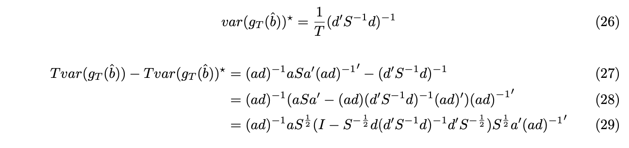
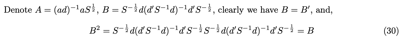
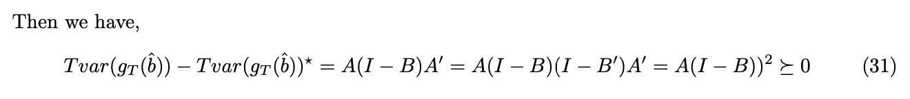
Under GMM framework, for each selection matrix a, we can find the consistent and asymptotically normal distributed estimator. However, which a leads to the most efficient GMM estimator still remains a question. We now show that with![]() , the estimator is efficient, by showing
, the estimator is efficient, by showing ![]() is positive semi-definite, where
is positive semi-definite, where ![]() is the variance of the estimator when
is the variance of the estimator when ![]() .
.
In Hansen’s paper, and perhaps also in a majority of textbooks, the GMM estimator is represented as follows,
![]()
Intuitively, the above objective function represents a “weighted norm” of the sample mean under ![]() . We’ll then show that, with new representation, the efficient
. We’ll then show that, with new representation, the efficient ![]() , is equivalent with the efficient
, is equivalent with the efficient ![]()
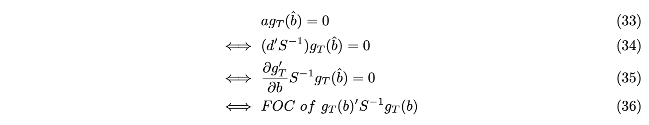
Therefore, ![]() is equivalent as
is equivalent as ![]() in corresponding settings, both reach the efficient GMM estimator.
in corresponding settings, both reach the efficient GMM estimator.
Under the efficient case, GMM estimators and test statistics can be simplified as follows,

Notice that the estimation of ![]() requires a or
requires a or ![]() . Meanwhile,
. Meanwhile, ![]() or
or ![]() depends on S, which again depends on
depends on S, which again depends on ![]() . In practice, people use two-staged GMM. First stage: set
. In practice, people use two-staged GMM. First stage: set ![]() , estimate
, estimate ![]() . Second stage: use
. Second stage: use ![]() to estimate S, then let
to estimate S, then let ![]() Re-calculate
Re-calculate ![]() to update the estimate. Second stage can be iterated several times until the result converges.
to update the estimate. Second stage can be iterated several times until the result converges.
As a simple application, GMM can be used to estimate linear model. We use the fact that the residual and right hand side variable are orthogonal.
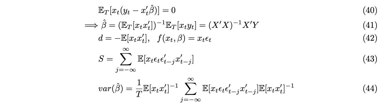
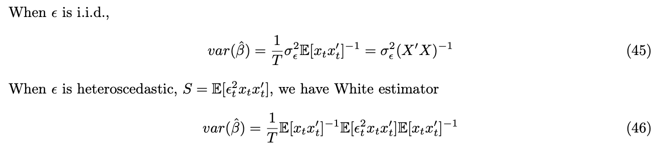
When ![]() is both heteroscedastic and autocorrelated, we have the famous Newey-West adjusted estimator with,
is both heteroscedastic and autocorrelated, we have the famous Newey-West adjusted estimator with,

Using the factor model as an example, now we form the following equation,

Although ![]() will give the most efficient estimation, in many cases, we should rather choose
will give the most efficient estimation, in many cases, we should rather choose ![]() based on the question we’re interested in, or the prior we have. For example, in the above case, our question is whether the pricing error of the CCAPM model is jointly zero on HML and SMB portfolios. Naturally, we shall set
based on the question we’re interested in, or the prior we have. For example, in the above case, our question is whether the pricing error of the CCAPM model is jointly zero on HML and SMB portfolios. Naturally, we shall set ![]() as shown above. It seems in this case, the selection of
as shown above. It seems in this case, the selection of ![]() may not be efficient. Indeed, as mentioned by Prof. Cochrane, although the GMM method provides as a strong tool in empirical asset pricing, it should not be treated as a black box. We should prevent such usage that by simply expressing the question with a series of moment conditions, and directly come up with an “efficient” estimate with GMM. What we should care is whether the efficient selection matrix makes sense, and whether it is able to align with the question of interest.
may not be efficient. Indeed, as mentioned by Prof. Cochrane, although the GMM method provides as a strong tool in empirical asset pricing, it should not be treated as a black box. We should prevent such usage that by simply expressing the question with a series of moment conditions, and directly come up with an “efficient” estimate with GMM. What we should care is whether the efficient selection matrix makes sense, and whether it is able to align with the question of interest.